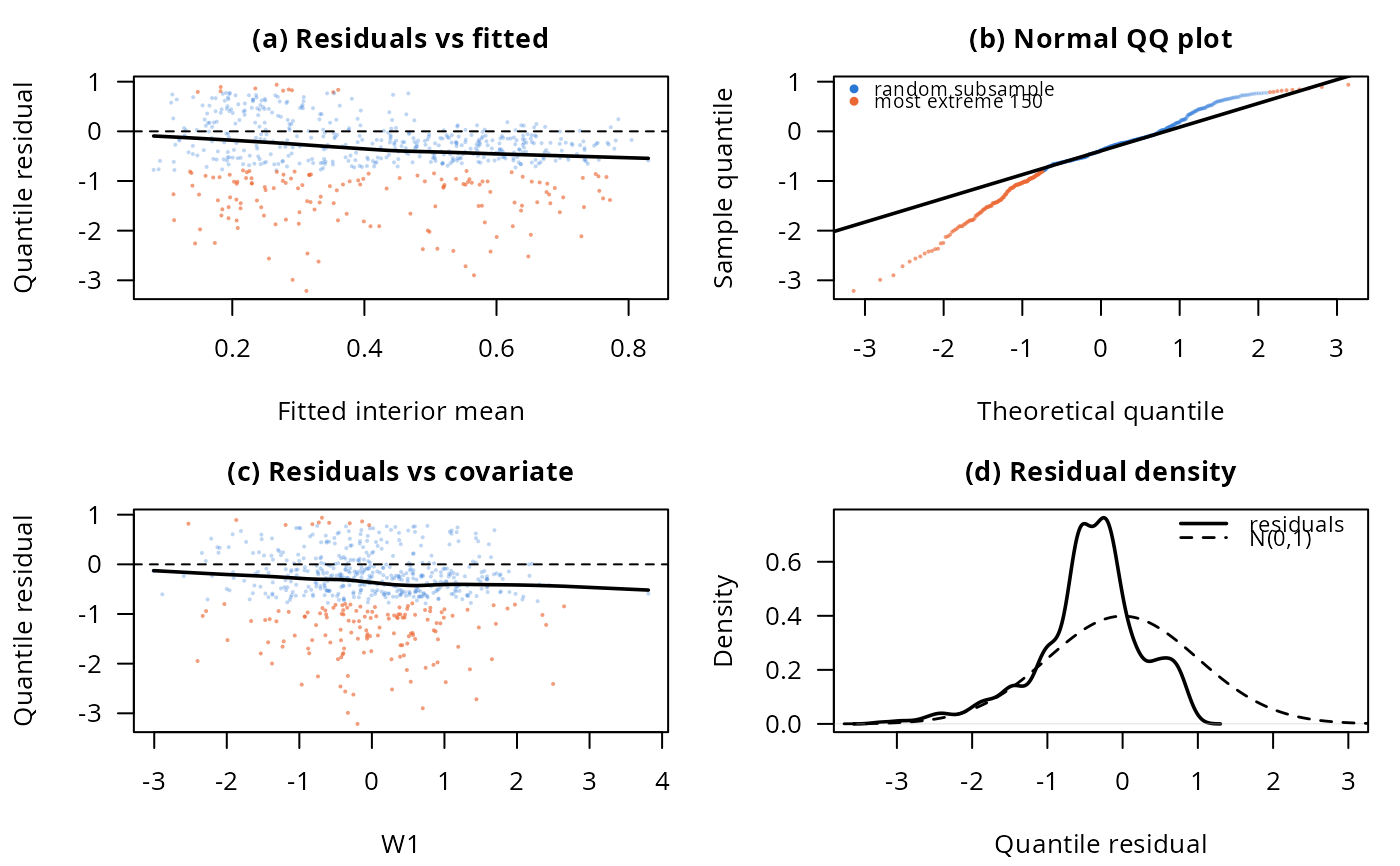
Goodness-of-fit diagnostics for a fitted BIc model (Figure 5 of Ospina, 2026)

Randomized quantile residuals (Dunn and Smyth, 1996) against the fitted mean and, optionally, a covariate, a normal QQ plot, and the residual density against the standard normal. Scatter panels subsample for plotting (the smoothers and all other statistics use the full data, since gamlss's residuals are unweighted even under survey weights, see Ospina (2026), Section 8.4): the subsample always keeps the n_extreme most extreme residuals, shown in orange, on top of a random draw of the rest, shown in blue, rather than a uniform random draw alone, which is biased toward hiding exactly the tail behavior a goodness-of-fit plot exists to show.

Usage

plot_diagnostics(
  fit,
  data,
  covariate = NULL,
  covariate_lab = covariate,
  n_extreme = 150,
  n_bulk = 8000,
  seed = NULL
)

Arguments

fit

A fitted model from bic_fit().

data

The data frame fit was fitted on.

covariate

Optional character, the name of a covariate in data to plot residuals against in an extra panel (used for the paper's log household income panel). NULL (default) omits that panel.

covariate_lab

Axis label for covariate's panel; defaults to covariate itself.

n_extreme

Number of most-extreme residuals always shown.

n_bulk

Size of the random subsample of the remaining residuals.

seed

Optional seed (randomized quantile residuals depend on it at the boundary observations; the paper fixes it).

Value

Invisibly, a list with residuals (the full vector of randomized quantile residuals), deviance, AIC, BIC, filliben (the probability-plot correlation coefficient) and shapiro (the shapiro.test() result on a random subsample of at most 5000, the largest the test accepts). Called mainly for its plotting side effect; draws all panels in the current graphics device.

Examples

dat <- simulate_bic(600, seed = 1)
fit <- bic_fit(y ~ T + W2, nu.formula = ~ T + W1, data = dat)
plot_diagnostics(fit, dat, covariate = "W1", seed = 1)