Reproducing the simulation study (Ospina, 2026)

This vignette reproduces the simulation study of Section 7 of Ospina (2026), using exactly the data-generating process and parameters of the manuscript’s paper2_simulation.R (the defaults of [simulate_bic()] are that same process). It runs end to end from package functions alone, with no external data.

library(causalbic)

What `tau_alpha` and `tau_mu` mean

Before looking at numbers: tau (the average treatment effect) is the total change in the mean response caused by treatment. tau_alpha is the part of that change coming from the treatment moving units onto or off the boundary (here, the probability of landing at y = 0); tau_mu is the part coming from the treatment shifting the conditional mean among units that remain in the interior. They always add up to tau exactly (see below), but they can, and in this design do, point in opposite directions, so a reader who only sees tau cannot tell whether the treatment acted on the boundary mechanism, the interior mechanism, both in agreement, or both in opposition with one dominating.

Population truth

The manuscript reports, from a population of $2\times10^6$ draws under gamma = c(-1.5, 0.3, 1.5), beta = c(-1.0, 0.5, 1.2), phi = 4, rho = 0.4: $\tau = 0.0463$ , $\tau_\alpha = -0.0876$ , $\tau_\mu = 0.1338$ . A large simulated population reproduces this closely:

set.seed(1)
pop <- simulate_bic(2e5, seed = 1)
unlist(attr(pop, "truth"))
#>         tau   tau_alpha      tau_mu 
#>  0.04630878 -0.08753647  0.13384524

Reading this substantively: the treatment actually increases the boundary probability ( $\tau_\alpha < 0$ here means a lower mean contribution from a higher chance of landing at the boundary, since the boundary is $y=0$ ) while it raises the interior mean enough to overcome that pull ( $\tau_\mu>0$ , and larger in magnitude than $\tau_\alpha$ ). The two components have opposite signs and are each about three times larger than their difference, $\tau$ : the average effect alone would describe this as a modest, roughly homogeneous effect and conceal that two mechanisms of comparable size are pulling in opposite directions.

Estimator behavior at finite samples

The manuscript’s Table 2 reports bias, RMSE and coverage at $n \in \{100, 200, 500\}$ over $R = 200$ replications. The loop below does the same at a smaller R, for vignette build time; set R <- 200 to reproduce Table 2 exactly (seeds match paper2_simulation.R).

run_once <- function(n, seed) {
  dat <- simulate_bic(n, seed = seed)
  fit <- bic_fit(y ~ T + W2, nu.formula = ~ T + W1, data = dat)
  bic_gcomp(fit, "T", dat)
}

R <- 20  ## paper uses R = 200
ns <- c(100, 200, 500)
truth <- unlist(attr(simulate_bic(10, seed = 1), "truth"))

results <- do.call(rbind, lapply(ns, function(n) {
  ests <- t(vapply(seq_len(R), function(r) run_once(n, seed = r), numeric(3)))
  bias <- colMeans(ests) - truth[c("tau", "tau_alpha", "tau_mu")]
  rmse <- sqrt(colMeans(sweep(ests, 2, truth[c("tau", "tau_alpha", "tau_mu")])^2))
  data.frame(n = n, bias_tau = bias["tau"], rmse_tau = rmse["tau"])
}))
rownames(results) <- NULL
results
#>     n      bias_tau   rmse_tau
#> 1 100  0.0104243005 0.05257762
#> 2 200  0.0041251320 0.04348827
#> 3 500 -0.0009232433 0.02760540

RMSE should decline roughly as $n^{-1/2}$ as $n$ grows, and bias should stay an order of magnitude below the effect size ( $\tau = 0.046$ ) at every $n$ , matching Table 2 of the manuscript. In practical terms, this table is the check that the estimator earns the right to be trusted on real data before Section 8 uses it there: a decomposition that looked exact algebraically but recovered the wrong $\tau_\alpha$ / $\tau_\mu$ split in finite samples would be a mathematical curiosity, not an estimator.

The decomposition is an exact identity

Regardless of R or n, the decomposition holds to floating-point precision on every single fit, not just on average:

dat <- simulate_bic(300, seed = 99)
fit <- bic_fit(y ~ T + W2, nu.formula = ~ T + W1, data = dat)
g <- bic_gcomp(fit, "T", dat)
g["tau"] - (g["tau_alpha"] + g["tau_mu"])
#> tau 
#>   0

This is not a numerical coincidence to be checked once and trusted: it follows from the inflated beta likelihood being separable (its Fisher information is block diagonal between the boundary-probability and mean submodels), so tau_alpha and tau_mu are not two separate estimates that happen to sum correctly, they are the same single fitted model read two ways. That is also why misspecifying the boundary submodel does not contaminate the mean submodel’s parameters (though it does bias the weight tau_mu is averaged with, since that weight is a boundary probability); see Section 4 of the manuscript.

Figures

causalbic also ships the plotting functions behind two of the manuscript’s figures, so they can be regenerated from the package alone, not just their underlying numbers. 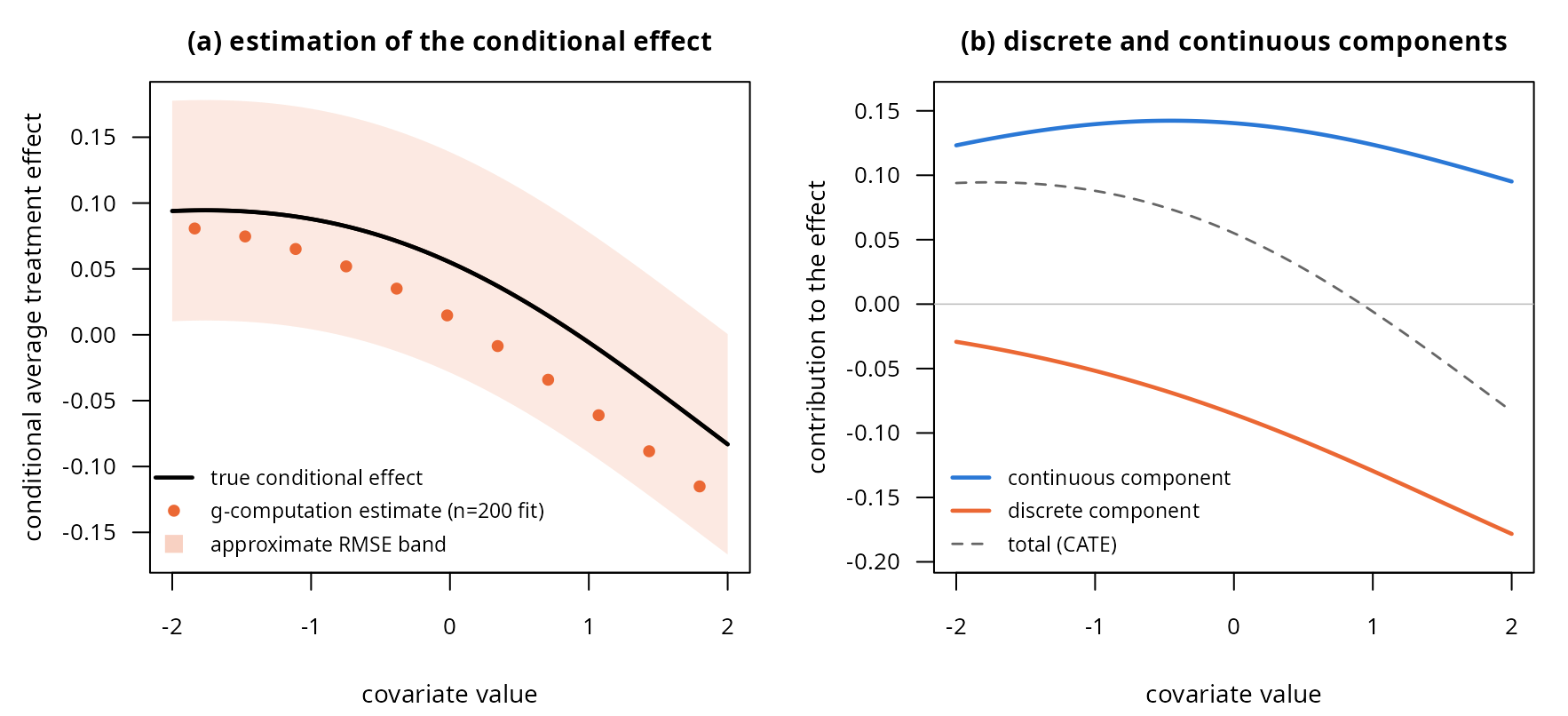Both are fully self-contained (no external data): [plot_concept()] draws the synthetic two-panel illustration of the discrete/continuous decomposition and the likelihood-displacement curve behind the causal curvature (Figure 1); [plot_cate()] simulates one dataset from the same process as above, fits it, and plots the true and estimated conditional average treatment effect alongside its two components (Figure 2).

par(mfrow = c(1, 2))
plot_concept()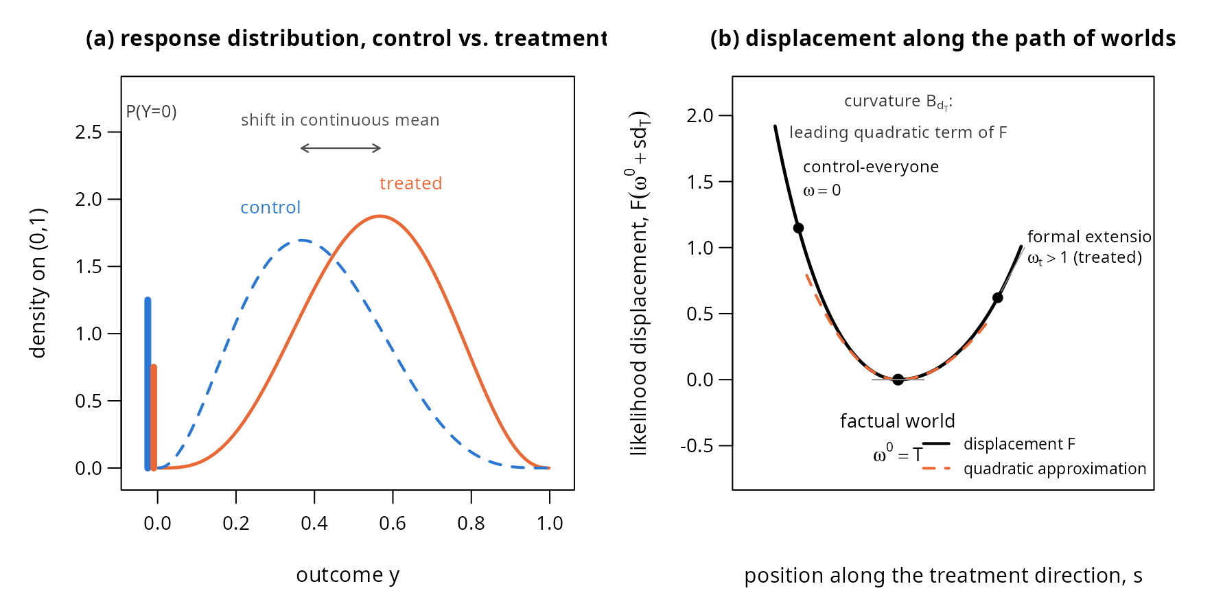

par(mfrow = c(1, 2))
invisible(plot_cate())

(A third figure, the application’s goodness-of-fit diagnostics, needs a fitted model on real data and is shown in vignette("paper-application") via [plot_diagnostics()].)

Reference