The conditional average treatment effect figure (Figure 2 of Ospina, 2026)

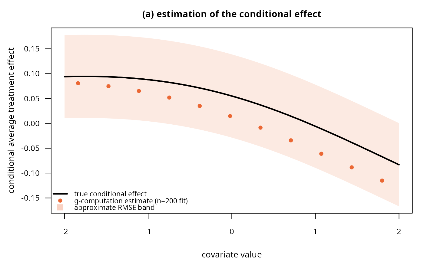
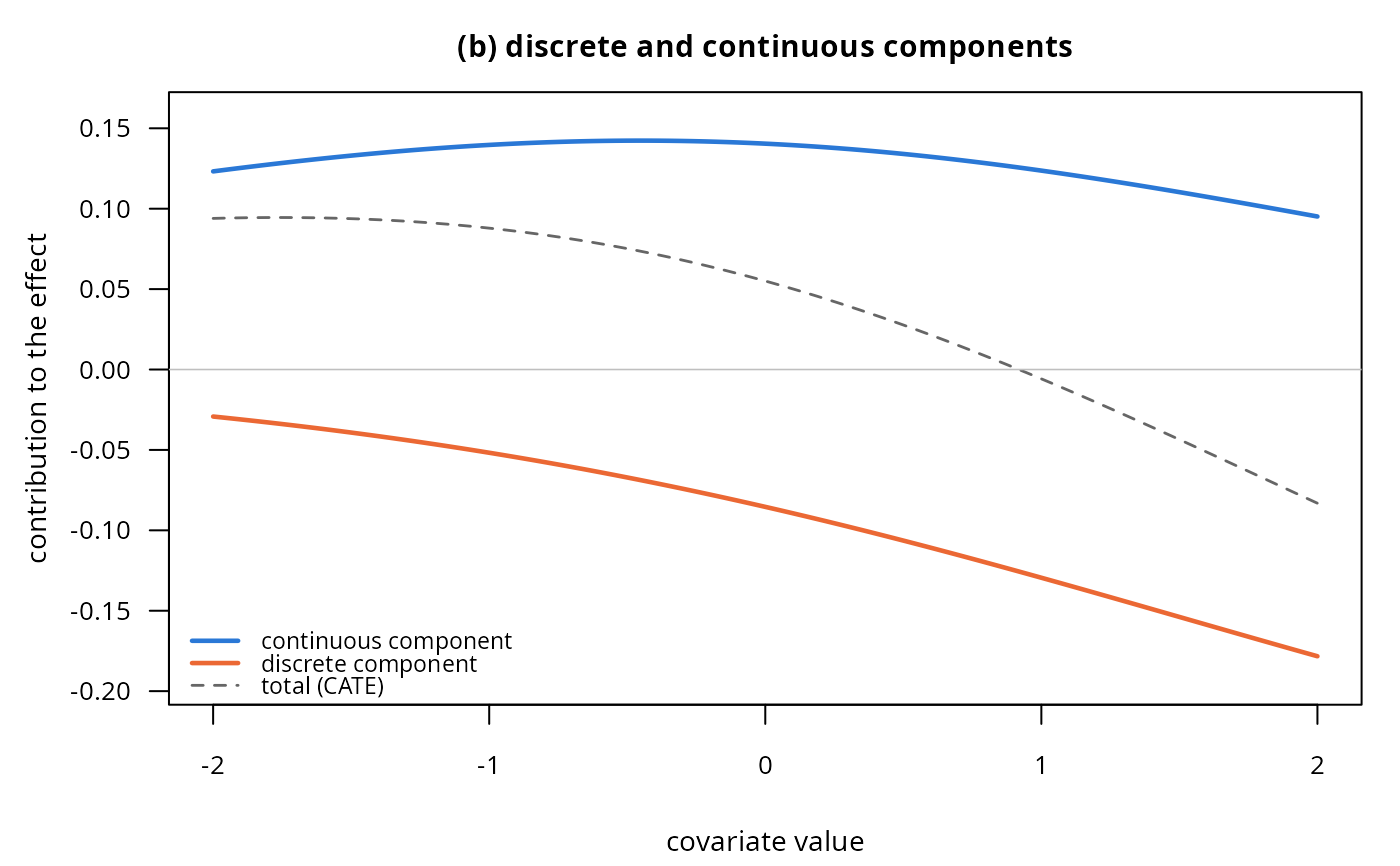
Simulates one dataset from simulate_bic(), fits it with bic_fit(), and plots (a) the true conditional average treatment effect (CATE) against the g-computation estimate from that single fit, with an RMSE band, and (b) the true discrete- and continuous-component contributions that add up to the CATE (the population-level counterpart of panel (b) of plot_concept()).

Usage

plot_cate(
  n = 200,
  seed = 7,
  gamma = c(-1.5, 0.3, 1.5),
  beta = c(-1, 0.5, 1.2),
  phi = 4,
  rho = 0.4,
  rmse = 0.0427
)

Arguments

n, seed, gamma, beta, phi, rho

As in simulate_bic(); the defaults reproduce the paper's figure exactly.

rmse

Half-width of the plotted uncertainty band around the true CATE in panel (a). Defaults to 0.0427, the R = 200-replicate, n = 200 root-mean-squared error at the median covariate profile reported in Table 2 of Ospina (2026); this is not recomputed by this function (that would need hundreds of refits), so pass your own value if you change n or the generating parameters.

Value

Invisibly, a list with grid (the covariate values plotted), truth (a data frame of tau, tau_alpha, tau_mu at each grid point) and estimate (the g-computation CATE from the single fitted model). Called mainly for its plotting side effect; draws both panels in the current graphics device (set par(mfrow = c(1, 2)) first).

Examples

plot_cate()