Growth-curve ensembles and phases of an epidemic

library(epicurves)

This vignette shows the functions behind the article on locating phase changes in epidemic curves (Ospina, Oliveira, Ferraz and Leite). The segmentation runs take one to several minutes each and are shown but not run.

Growth curves on daily counts

A cumulative growth curve $C(u)$ implies the daily mean $\mu_u = C(u) - C(u-1)$. fit_growth_incidence() fits one curve to daily counts by Poisson or negative binomial likelihood, and fit_ensemble_incidence() fits the Logistic, Gompertz and Richards curves and combines them with Akaike weights.

u <- 1:100
mu <- growth_incidence(u, "gompertz", y0 = 10, K = 3000, gamma = 0.05)
set.seed(1)
x <- rpois(100, mu)
ens <- fit_ensemble_incidence(x, family = "poisson")
round(ens$weights, 3)
#> gompertz richards logistic 
#>        1        0        0
plot(u, x, pch = 19, cex = 0.6, xlab = "Day", ylab = "Daily count")
lines(u, predict(ens, u), lwd = 2)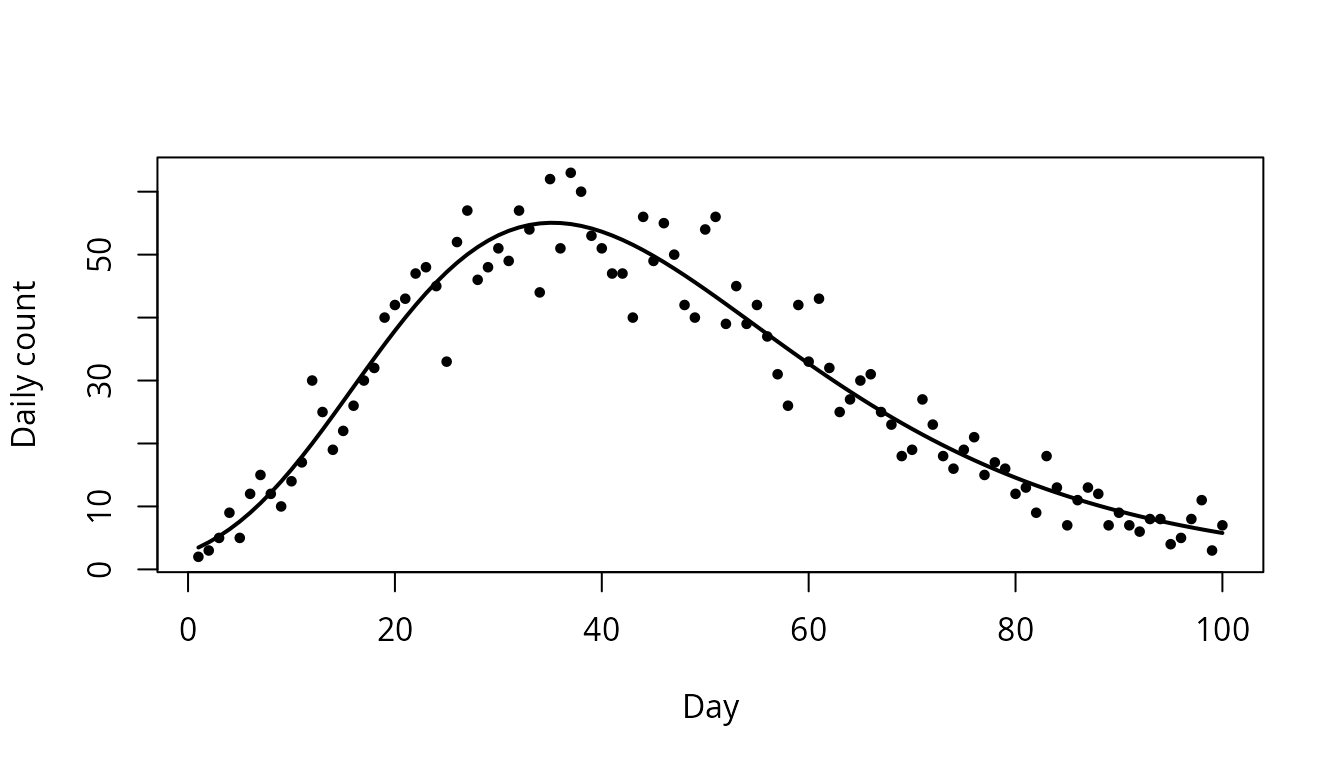

Dividing a series into phases

bic_segment() divides a completed series by binary segmentation with a penalised likelihood on the daily scale. edetect_segment() monitors the series as it arrives with two one-sided e-detectors (package edetect), which compare each count with a band around the forecast of the current phase and bound the probability of a false alarm at any time when the band contains the conditional mean. With z = 0 the band is the point forecast itself; a band of one standard error (z = 1) allows for the error in the forecast.

data(paraiba_covid19)
deaths <- paraiba_covid19$new_deaths
seg <- bic_segment(deaths, d_min = 12, family = "negbin", step = 5)
paraiba_covid19$date[seg$cuts]
det <- edetect_segment(deaths, d_min = 20, arl = 1000, refit_every = 7,
                       chart = "subgaussian", z = 1)
paraiba_covid19$date[det$cuts]
paraiba_covid19$date[det$alarms]

For overdispersed counts, use the negative binomial family in bic_segment() and the sub-Gaussian chart in edetect_segment(); with the Poisson chart, daily case counts whose variance far exceeds their mean are read as a sequence of changes.

The earlier approach on cumulative counts

fit_piecewise_ensemble() implements the earlier rule, which fits the curves to cumulative counts by least squares and accepts a split when it halves the mean squared error (confirm_criterion = "mse_threshold") or lowers a BIC computed from the cumulative residuals (confirm_criterion = "aic"). In the simulation study of the article both variants divided series generated by a single growth curve into several phases, because the errors of a cumulative series are strongly autocorrelated; the functions are kept to reproduce the earlier analyses.