Getting started with logcumulant • logcumulant

library(logcumulant)
data(reliability_datasets)

Why log-cumulants?

For positive-support data the Mellin transform plays the role that the Fourier or Laplace transform plays on the whole line. Differentiating the Mellin characteristic function at its central point yields the log-cumulants $\kappa_1, \kappa_2, \ldots$ : the cumulants of $\log X$ . These quantities are natural shape descriptors for reliability distributions and behave well under the multiplicative structure typical of lifetime data.

The package turns these descriptors into (i) diagnostic diagrams and (ii) formal goodness-of-fit tests.

A first analysis

We use the classic ball-bearing fatigue-life dataset bundled with the package.

bb <- reliability_datasets$BallBearing
length(bb)
#> [1] 23
summary(bb)
#>    Min. 1st Qu.  Median    Mean 3rd Qu.    Max. 
#>   17.88   47.04   67.80   72.22   95.88  173.40

The quickest entry point is plot_lc(), which draws the log-cumulant diagram with a bootstrap cloud of the sample estimate:

plot_lc(bb, B = 200)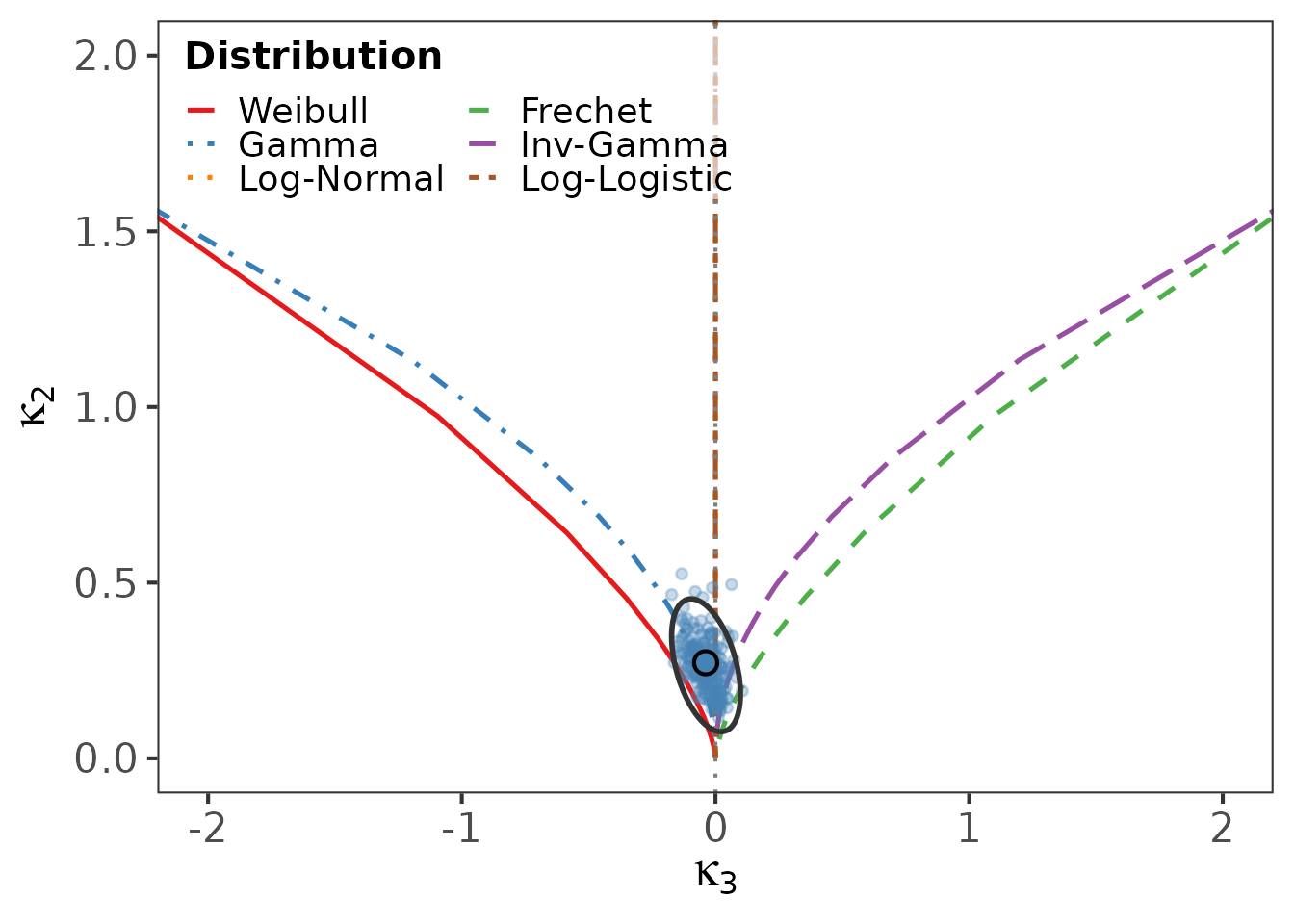

The sample point sits near the Weibull and Gamma loci, suggesting a light-tailed model.

Comparing candidate models

gof_compare_all() fits all six families and reports the three $T^2$ statistics, the Anderson–Darling and Cramer–von Mises tests, and the AIC. The parametric bootstrap is recommended for the p-values:

gof_compare_all(bb, use_bootstrap = TRUE, B = 199, seed = 1)
#>              Dist     T2_23      p_23      T2_123        p_123    T2_full
#> stat      Weibull 1.7684442 0.1835747   4.1163555 1.276864e-01 12.4859496
#> stat1     Frechet 1.3820542 0.2397516 269.3727725 3.209561e-59 79.9397649
#> stat2       Gamma 0.4802072 0.4883285   0.4003921 8.185703e-01  0.8889327
#> stat3    InvGamma 0.9577940 0.3277433   4.6352936 9.850512e-02  5.5465619
#> stat4   LogNormal 0.2566868 0.6124055   0.3937496 8.212935e-01  2.6732346
#> stat5 LogLogistic 0.2275893 0.6333171   0.2440233 8.851381e-01  3.6104646
#>             p_full        AD      AD_p        CvM     CvM_p      AIC     pb_23
#> stat  1.408080e-02 0.3285906 0.9152403 0.05795851 0.8268379 231.3826 0.3316583
#> stat1 1.793764e-16 0.5755471 0.6714156 0.07790501 0.7040599 235.5642 0.4572864
#> stat2 9.261432e-01 0.2153670 0.9856293 0.03909866 0.9377403 230.0586 0.5728643
#> stat3 2.356669e-01 0.3140940 0.9272090 0.04229426 0.9209759 232.3086 0.3567839
#> stat4 6.139063e-01 0.1888150 0.9931619 0.02896580 0.9794400 230.2571 0.6130653
#> stat5 4.612819e-01 0.1957724 0.9915227 0.03269626 0.9664924 230.7445 0.8040201
#>          pb_123   pb_full
#> stat  0.1758794 0.4321608
#> stat1 0.0000000 0.1256281
#> stat2 0.5276382 0.9849246
#> stat3 0.1005025 0.5527638
#> stat4 0.4522613 0.8040201
#> stat5 0.7236181 0.7487437

Where to go next

vignette("diagrams") explains the three diagnostic diagrams.
vignette("gof-tests") covers the tests and why the bootstrap is needed.
vignette("simulation") reproduces the size and power studies.