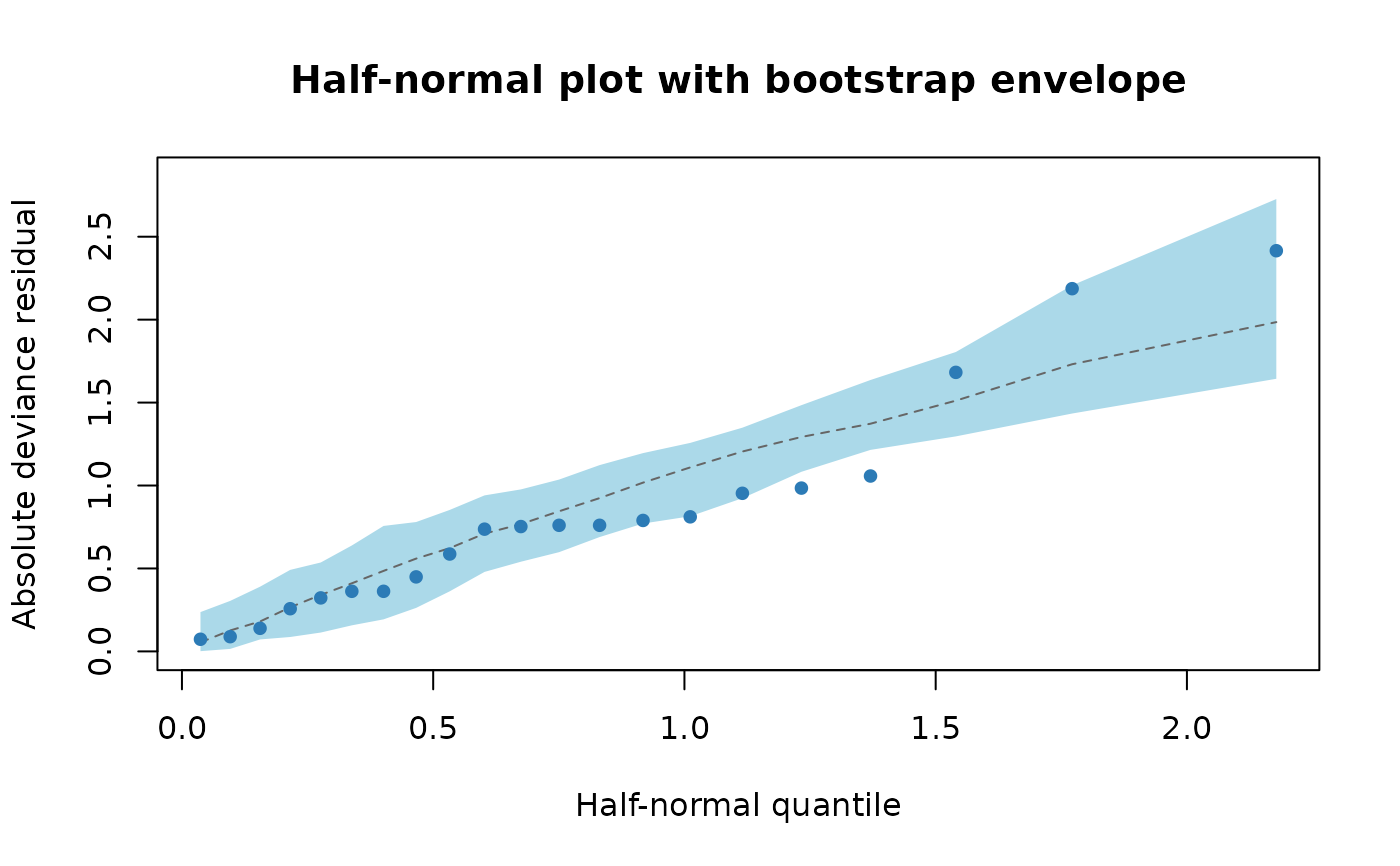
Half-Normal Probability Plot with Simulated Envelope

Produces a half-normal plot (Atkinson, 1985) with a simulated envelope of absolute deviance residuals with a bootstrap envelope, used to assess the overall fit of a simplex regression model. This replicates the diagnostic plots in Ospina et al. (2026).

Usage

plot_envelope(
  fit,
  B = 99,
  conf = 0.95,
  col.obs = "#2c7bb6",
  col.env = "#abd9e9",
  main = "Half-normal plot with bootstrap envelope",
  xlab = "Half-normal quantile",
  ylab = "Absolute deviance residual",
  ...
)

Arguments

fit: A "simplexfit" object.
B: Integer; number of simulations for the envelope. Default 99.
conf: Numeric in (0,1); confidence level for the envelope. Default 0.95.
col.obs: Colour for the observed residuals.
col.env: Colour for the envelope band.
main, xlab, ylab: Plot labels.
...: Further arguments to plot.

Value

Invisibly returns a list with $residuals (observed) and $envelope (matrix of simulated residuals).

References

Atkinson A.C. (1985). Plots, Transformations, and Regression. Oxford University Press.

Examples

data(ammonia)
X <- cbind(1, ammonia$corr_ar, ammonia$temp_agua,
           ammonia$corr_ar * ammonia$temp_agua)
Z <- cbind(1, ammonia$temp_agua,
           ammonia$corr_ar * ammonia$temp_agua)
fit <- simplex_fit(ammonia$perda, X, Z)
plot_envelope(fit, B = 99)