Paper: PBSC application

library(simplexgof)

The PBSC application

This article reproduces the peripheral blood stem cell (PBSC) transplantation application from the companion methodological paper (Ospina, Espinheira, Silva and Barros, 2026), using the pbsc dataset (Edmonton Hematopoietic Institute - Alberta Health Services).

The response recovery is the CD34+ cell recovery rate, a continuous proportion in $(0, 1)$. The constant-dispersion model used in paper_pbsc() is

$$\mathrm{logit}(\mu_t) = \beta_1 + \beta_2\,\mathrm{adj\_age}_t + \beta_3\,\mathrm{chemo}_t$$

$$\log(\sigma^2_t) = \gamma_1$$

where adj_age is the adjusted patient-age variable and chemo is the chemotherapy protocol indicator (0 = one-day, 1 = three-day protocol).

The data

data(pbsc)
head(pbsc)
#>   recovery adj_age chemo
#> 1     0.75      22     0
#> 2     0.83       0     1
#> 3     0.94       3     1
#> 4     0.86      18     0
#> 5     0.54       3     0
#> 6     0.70      11     1
summary(pbsc)
#>     recovery         adj_age          chemo       
#>  Min.   :0.4000   Min.   : 0.00   Min.   :0.0000  
#>  1st Qu.:0.7250   1st Qu.: 4.00   1st Qu.:0.0000  
#>  Median :0.8000   Median :16.00   Median :0.0000  
#>  Mean   :0.7907   Mean   :13.77   Mean   :0.4561  
#>  3rd Qu.:0.8700   3rd Qu.:22.00   3rd Qu.:1.0000  
#>  Max.   :0.9900   Max.   :31.00   Max.   :1.0000

One-call reproduction

The function paper_pbsc() fits the model, runs the bootstrap GoF test, and produces the diagnostic plots from the paper in a single call. We use B = 50 bootstrap replicates here for speed; the paper uses B = 1000.

res <- paper_pbsc(B = 50, seed = 456, plot = TRUE, verbose = FALSE)

Parameter estimates

print(res$table_params, row.names = FALSE)
#>  Parameter  Sub_model Estimate Std_Error z_value p_value
#>      beta1       Mean   1.1002    0.1401  7.8531  <0.001
#>      beta2       Mean   0.0136    0.0065  2.0913  0.0365
#>      beta3       Mean   0.2661    0.1245  2.1381  0.0325
#>     gamma1 Dispersion   1.8558    0.0915 20.2865  <0.001

Goodness-of-fit results

print(res$table_gof, row.names = FALSE)
#>      Un alpha Boot_lo Boot_hi    Decision_boot Norm_lo Norm_hi    Decision_norm
#>  0.2953    1% -0.8183  0.4329 Do not reject H0 -2.5758  2.5758 Do not reject H0
#>  0.2953    5% -0.7492  0.3526 Do not reject H0 -1.9600  1.9600 Do not reject H0
#>  0.2953   10% -0.7308  0.1987        Reject H0 -1.6449  1.6449 Do not reject H0

Step by step

X <- cbind(1, pbsc$adj_age, pbsc$chemo)
colnames(X) <- c("(Intercept)", "adj_age", "chemo")
Z <- matrix(1, nrow(pbsc), 1)
colnames(Z) <- "(Intercept)"

fit <- simplex_fit(pbsc$recovery, X, Z)
fit
#> 
#> Simplex Regression  (n = 239 ; p = 3 ; q = 1 )
#> 
#>        Estimate Std.Error z.value     Pr
#> beta1    1.1002    0.1401  7.8531 <0.001
#> beta2    0.0136    0.0065  2.0913 0.0365
#> beta3    0.2661    0.1245  2.1381 0.0325
#> gamma1   1.8558    0.0915 20.2865 <0.001
#> 
#> Log-likelihood: 156.6241  |  converged: TRUE

dg <- simplex_diag(fit)
dg$Tn
#> [1] 94.31959
dg$Un
#> [1] 0.2953172

plot_influence(dg)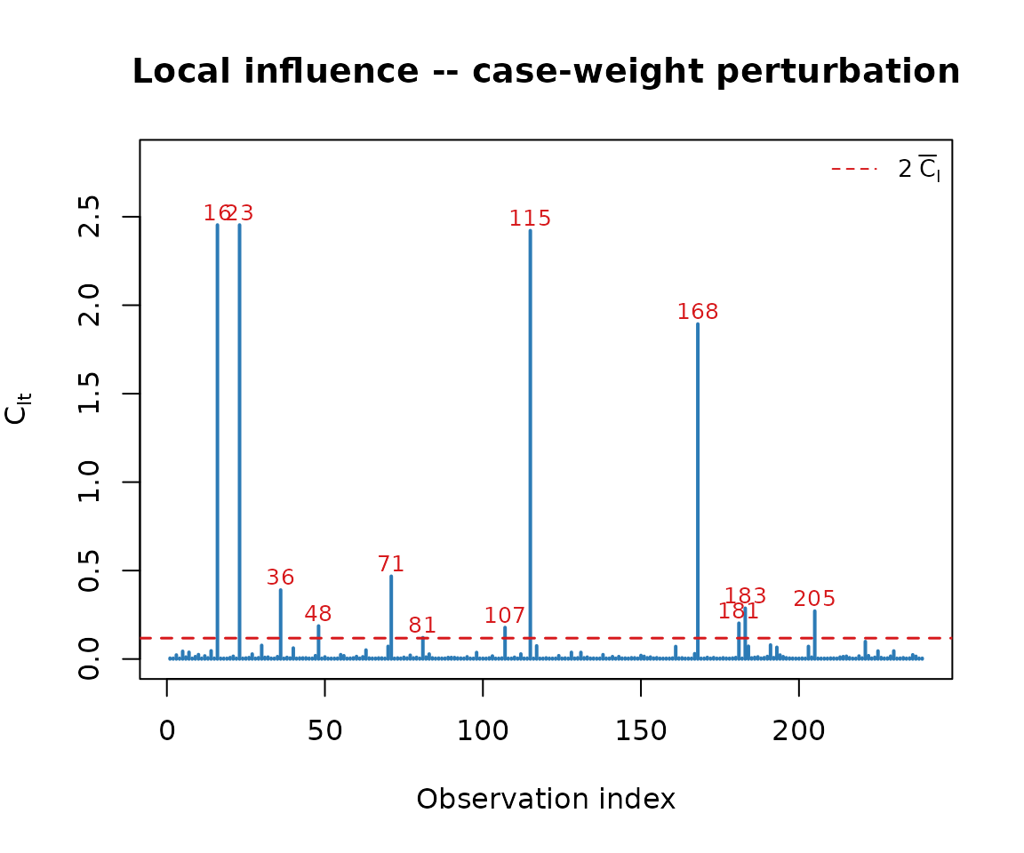

set.seed(456)
gof <- simplex_gof(pbsc$recovery, X, Z, B = 50, verbose = FALSE)
gof
#> simplexgof: U_n = 0.2953  (Tn = 94.3196, B = 50)
#> 
#>  alpha boot_lo boot_hi    decision_boot norm_lo norm_hi    decision_norm
#>     1% -0.8183  0.4329 Do not reject H0 -2.5758  2.5758 Do not reject H0
#>     5% -0.7492  0.3526 Do not reject H0 -1.9600  1.9600 Do not reject H0
#>    10% -0.7308  0.1987        Reject H0 -1.6449  1.6449 Do not reject H0

plot_gof_boot(gof)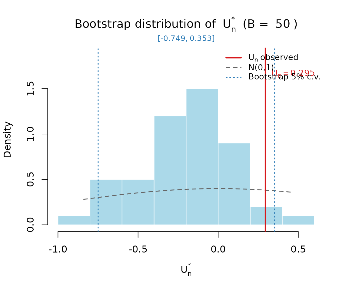

With $n = 242$, this larger sample illustrates the bootstrap calibration in a setting where the asymptotic approximation is already reasonably well behaved, and serves as a useful contrast with the small-sample ammonia application.

References

Ospina, R., Espinheira, P. L., Silva, F. C., Barros, M. (2026). A Bootstrap-Calibrated Local Influence Goodness-of-Fit Procedure for Simplex Regression Models.