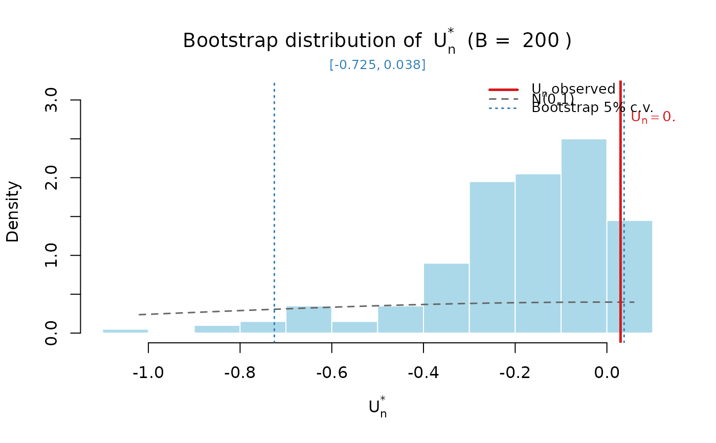
Displays the empirical bootstrap distribution of \(U_n^*\) together with the observed value \(U_n\) and the bootstrap critical values at each significance level, as shown in Ospina et al. (2026).
Usage
plot_gof_boot(
  x,
  col.hist = "#abd9e9",
  col.obs = "#d7191c",
  col.cv = "#2c7bb6",
  main = NULL,
  xlab = expression(U[n]^"*"),
  ylab = "Density",
  ...
)
Arguments
- x
A
"simplexgof"object fromsimplex_gof.- col.hist
Fill colour for the histogram.
- col.obs
Colour for the observed \(U_n\) line.
- col.cv
Colour for the critical-value lines.
- main, xlab, ylab
Plot labels.
- ...
Further arguments passed to
hist.
Examples
# \donttest{
data(ammonia)
X <- cbind(1, ammonia$corr_ar, ammonia$temp_agua,
           ammonia$corr_ar * ammonia$temp_agua)
Z <- cbind(1, ammonia$temp_agua,
           ammonia$corr_ar * ammonia$temp_agua)
set.seed(123)
gof <- simplex_gof(ammonia$perda, X, Z, B = 200, verbose = FALSE)
plot_gof_boot(gof)

# }
# }