Paper: ammonia application

library(simplexgof)

The ammonia application

This article reproduces the ammonia-oxidation application from the companion methodological paper (Ospina, Espinheira, Silva and Barros, 2026), using the ammonia dataset (Brownlee, 1965; $n = 21$).

The model fitted in the paper has

$$\mathrm{logit}(\mu_t) = \beta_1 + \beta_2 x_{t2} + \beta_3 x_{t3} + \beta_4 x_{t2} x_{t3}$$

for the mean, and

$$\log(\sigma^2_t) = \gamma_1 + \gamma_2 x_{t3} + \gamma_3 x_{t2} x_{t3}$$

for the dispersion, where $x_{t2}$ = corr_ar (air flow) and $x_{t3}$ = temp_agua (cooling water inlet temperature).

One-call reproduction

The function paper_ammonia() fits this model, runs the bootstrap GoF test, and produces the diagnostic plots from the paper in a single call. We use B = 50 bootstrap replicates here for speed; the paper uses B = 1000.

res <- paper_ammonia(B = 50, seed = 123, plot = TRUE, verbose = FALSE)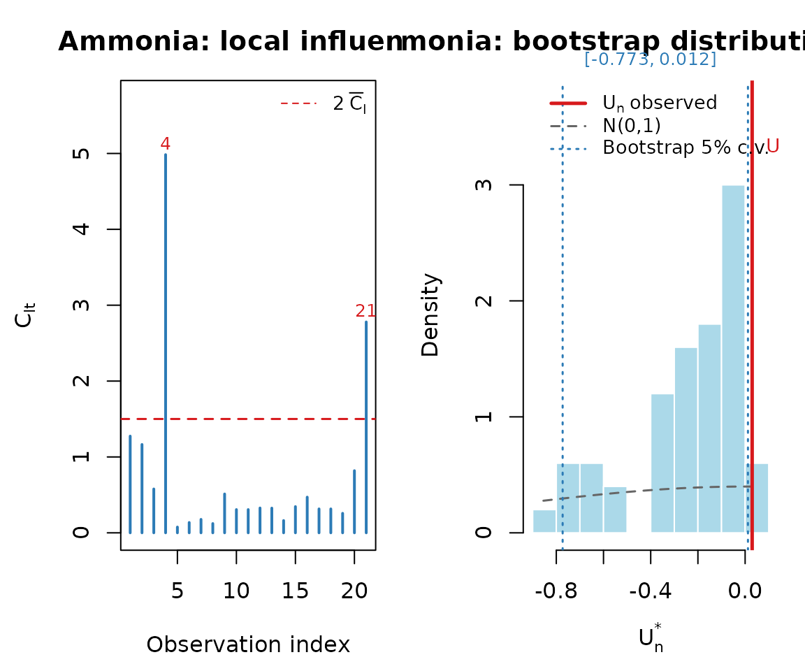

Parameter estimates (Table 5 of the paper)

print(res$table_params, row.names = FALSE)
#>  Parameter  Sub_model Estimate Std_Error z_value p_value
#>      beta1       Mean -12.9893    2.1038 -6.1742 < 0.001
#>      beta2       Mean   0.1312    0.0363  3.6140 < 0.001
#>      beta3       Mean   0.2705    0.1024  2.6408 0.00827
#>      beta4       Mean  -0.0037    0.0017 -2.1473 0.03177
#>     gamma1 Dispersion   3.8342    3.3908  1.1308 0.25815
#>     gamma2 Dispersion  -0.4454    0.2882 -1.5456 0.12219
#>     gamma3 Dispersion   0.0044    0.0024  1.8791 0.06024

Goodness-of-fit results (Table 6 of the paper)

print(res$table_gof, row.names = FALSE)
#>      Un alpha Boot_lo Boot_hi Decision_boot Norm_lo Norm_hi    Decision_norm
#>  0.0298    1% -0.8371  0.0255     Reject H0 -2.5758  2.5758 Do not reject H0
#>  0.0298    5% -0.7731  0.0120     Reject H0 -1.9600  1.9600 Do not reject H0
#>  0.0298   10% -0.7330 -0.0010     Reject H0 -1.6449  1.6449 Do not reject H0

Step by step

The same analysis can be reproduced manually with the lower-level functions of the package:

data(ammonia)

X <- cbind(1, ammonia$corr_ar, ammonia$temp_agua,
           ammonia$corr_ar * ammonia$temp_agua)
Z <- cbind(1, ammonia$temp_agua,
           ammonia$corr_ar * ammonia$temp_agua)

fit <- simplex_fit(ammonia$perda, X, Z)
fit
#> 
#> Simplex Regression  (n = 21 ; p = 4 ; q = 3 )
#> 
#>        Estimate Std.Error z.value      Pr
#> beta1  -12.9893    2.1038 -6.1742 < 0.001
#> beta2    0.1312    0.0363  3.6140 < 0.001
#> beta3    0.2705    0.1024  2.6408 0.00827
#> beta4   -0.0037    0.0017 -2.1473 0.03177
#> gamma1   3.8342    3.3908  1.1308 0.25815
#> gamma2  -0.4454    0.2882 -1.5456 0.12219
#> gamma3   0.0044    0.0024  1.8791 0.06024
#> 
#> Log-likelihood: 100.4159  |  converged: TRUE

dg <- simplex_diag(fit)
dg$Tn
#> [1] 8.044735
dg$Un
#> [1] 0.02977546

plot_influence(dg)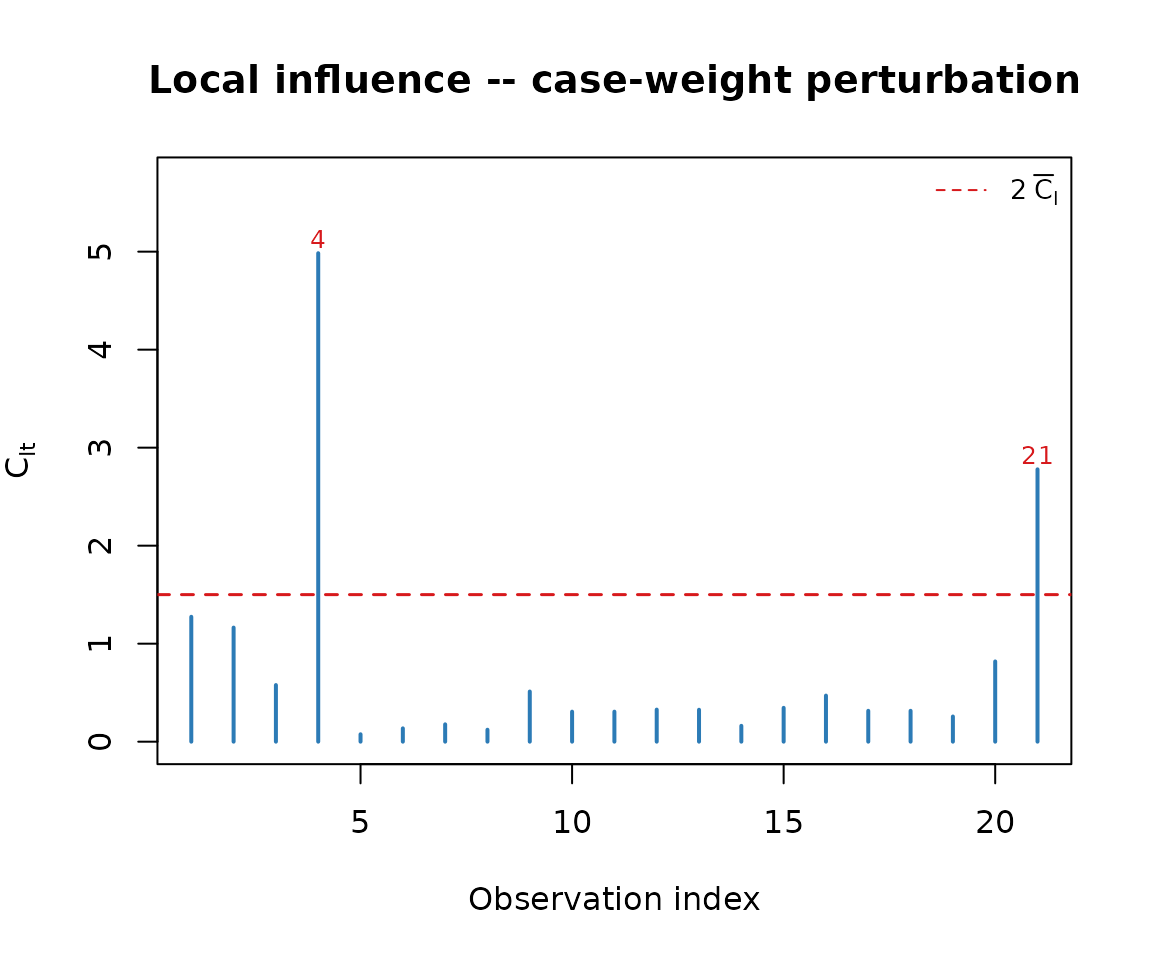

set.seed(123)
gof <- simplex_gof(ammonia$perda, X, Z, B = 50, verbose = FALSE)
gof
#> simplexgof: U_n = 0.0298  (Tn = 8.0447, B = 50)
#> 
#>  alpha boot_lo boot_hi decision_boot norm_lo norm_hi    decision_norm
#>     1% -0.8371  0.0255     Reject H0 -2.5758  2.5758 Do not reject H0
#>     5% -0.7731  0.0120     Reject H0 -1.9600  1.9600 Do not reject H0
#>    10% -0.7330 -0.0010     Reject H0 -1.6449  1.6449 Do not reject H0

plot_gof_boot(gof)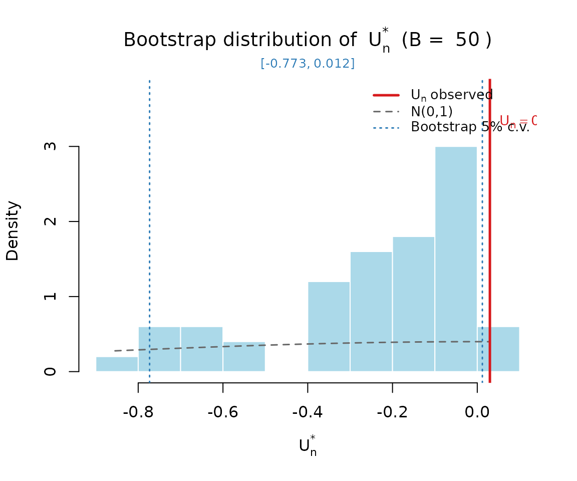

As reported in the paper, the test does not reject $H_0$ at conventional significance levels for this model, consistent with an adequate fit.

References

Brownlee, K. A. (1965). Statistical Theory and Methodology in Science and Engineering. Wiley.

Ospina, R., Espinheira, P. L., Silva, F. C., Barros, M. (2026). A Bootstrap-Calibrated Local Influence Goodness-of-Fit Procedure for Simplex Regression Models.