Introduction to simplexgof

library(simplexgof)

Overview

simplexgof implements a bootstrap-calibrated local-influence goodness-of-fit (GoF) test for simplex regression models with constant or varying dispersion. The package provides:

• simplex_fit(): fit a simplex regression model via maximum likelihood, with logit link for the mean and log link for the dispersion.
• simplex_diag(): compute local-influence diagnostic quantities (the $T_n$ and $U_n$ statistics, individual influence measures $C_{I_t}$).
• simplex_gof(): run the full parametric-bootstrap GoF test.
• Plotting functions to visualise influence diagnostics, half-normal envelopes, and the bootstrap distribution of $U_n$.

This vignette walks through a complete analysis using the ammonia dataset bundled with the package.

The data

The ammonia dataset (Brownlee, 1965) has 21 observations on the proportion of ammonia lost during an industrial oxidation process, together with three covariates.

data(ammonia)
head(ammonia)
#>   perda corr_ar temp_agua conc_acido
#> 1 0.042      80        27         89
#> 2 0.037      80        27         88
#> 3 0.037      75        25         90
#> 4 0.028      62        24         87
#> 5 0.018      62        22         87
#> 6 0.018      62        23         87

The response perda is a proportion in $(0, 1)$, making it a natural candidate for simplex regression.

Fitting a simplex regression model

We model the mean $\mu_t$ with covariates corr_ar, temp_agua, and their interaction, and allow the dispersion $\sigma^2_t$ to depend on temp_agua and the same interaction term.

X <- cbind(1, ammonia$corr_ar, ammonia$temp_agua,
           ammonia$corr_ar * ammonia$temp_agua)
Z <- cbind(1, ammonia$temp_agua,
           ammonia$corr_ar * ammonia$temp_agua)

fit <- simplex_fit(ammonia$perda, X, Z)
fit
#> 
#> Simplex Regression  (n = 21 ; p = 4 ; q = 3 )
#> 
#>        Estimate Std.Error z.value      Pr
#> beta1  -12.9893    2.1038 -6.1742 < 0.001
#> beta2    0.1312    0.0363  3.6140 < 0.001
#> beta3    0.2705    0.1024  2.6408 0.00827
#> beta4   -0.0037    0.0017 -2.1473 0.03177
#> gamma1   3.8342    3.3908  1.1308 0.25815
#> gamma2  -0.4454    0.2882 -1.5456 0.12219
#> gamma3   0.0044    0.0024  1.8791 0.06024
#> 
#> Log-likelihood: 100.4159  |  converged: TRUE

The fitted object has class "simplexfit", with print, coef, and fitted methods.

coef(fit)
#>         beta1         beta2         beta3         beta4        gamma1 
#> -12.989277095   0.131221084   0.270456444  -0.003688490   3.834204684 
#>        gamma2        gamma3 
#>  -0.445382852   0.004442287

Influence diagnostics

simplex_diag() computes the case-weight local-influence measures $C_{I_t}$ and the test statistics $T_n$ and $U_n$ that aggregate them.

dg <- simplex_diag(fit)
dg$Tn
#> [1] 8.044735
dg$Un
#> [1] 0.02977546

These quantities can be visualised with plot_influence(), which produces an index plot of the individual influence values $C_{I_t}$:

plot_influence(dg)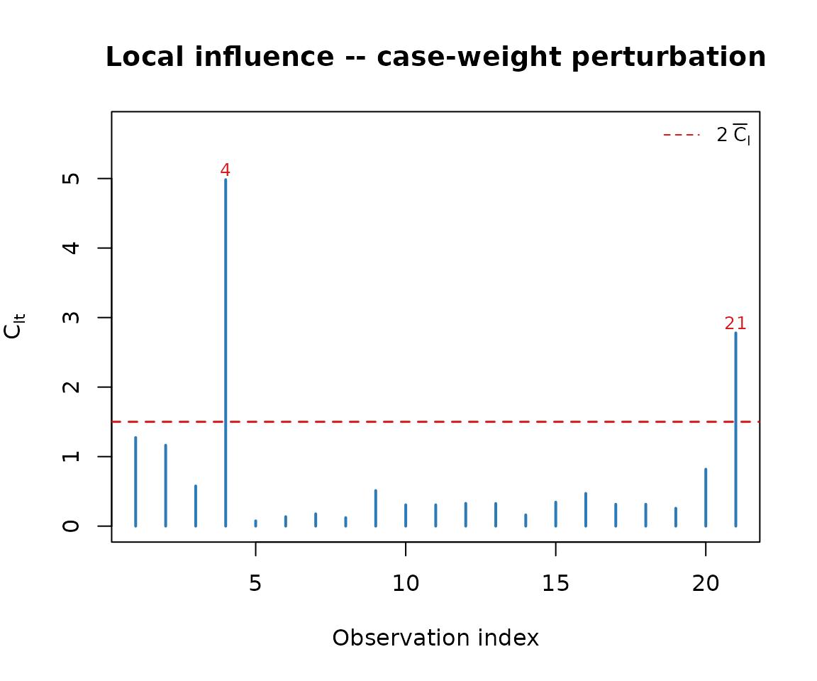

The bootstrap goodness-of-fit test

Because the first-order asymptotic normal calibration of $U_n$ is known to be liberal in small samples, simplex_gof() provides a parametric bootstrap calibration. With B = 50 replicates (for speed in this vignette; use a larger B, e.g. 1000, in practice):

set.seed(42)
gof <- simplex_gof(ammonia$perda, X, Z, B = 50, alpha = 0.01,
                    verbose = FALSE)
gof
#> simplexgof: U_n = 0.0298  (Tn = 8.0447, B = 50)
#> 
#>  alpha boot_lo boot_hi    decision_boot norm_lo norm_hi    decision_norm
#>     1% -0.8248  0.0424 Do not reject H0 -2.5758  2.5758 Do not reject H0

The bootstrap distribution of $U_n$ under $H_0$ can be visualised with plot_gof_boot():

plot_gof_boot(gof)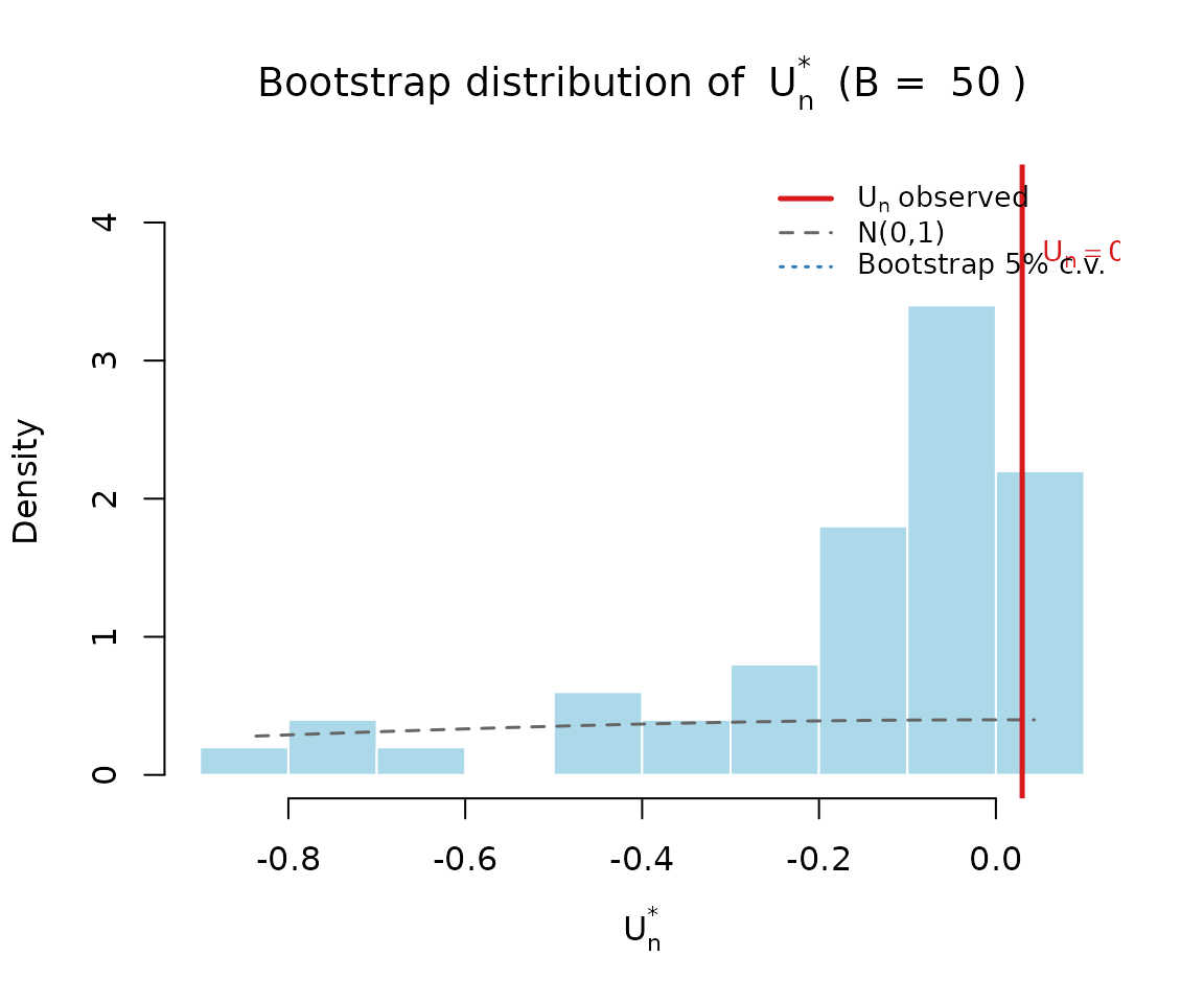

Half-normal plot with simulated envelope

plot_envelope() produces a half-normal plot of the influence measures with a simulated envelope, useful for spotting individual observations that drive the lack of fit:

plot_envelope(fit, B = 99)

Convenience plot methods

Both "simplexfit" and "simplexgof" objects have plot() methods that wrap the functions above:

plot(fit, which = "influence")
plot(gof, which = "boot")

Next steps

For full reproductions of the figures and tables in the companion methodological paper (Ospina, Espinheira, Silva and Barros, 2026), see the “Paper: ammonia application” and “Paper: PBSC application” articles.